Part 3

As seen in Part 2 in the GA Schema, the first step of a high-level representation of a GA is initializing the population of chromosomes (individuals). Therefore, in this part, we’ll talk about chromosomal representation and begin with hands-on implementation using one of the most classic forms of representation: binary.

Chromosomal Representation

A chromosomal representation is necessary to describe each individual in the GA population. The representation scheme determines how the problem is structured in the GA. In summary, chromosomal representation provides a way to translate the information of our problem into a form that a computer can handle.

As seen in Part 2, each chromosome is composed of a sequence of genes. A gene is the smallest portion that makes up a chromosome.

There are a few general rules that should be followed when creating a new representation:

1. Keep it as simple as possible;
2. If there are forbidden solutions to our problem, it’s preferable not to have a representation for such a solution;
3. If there are conditions in our problem, they should be implicit within the chosen representation.

One of the most widely used representations is a binary representation, and this will be the one adopted throughout our series. Binary chromosomal representation consists of a sequence where each gene takes the values 1 and 0, as shown in the following image.

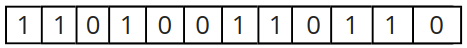
But what does each gene (or bit) represent?

Each of these genes, or a set of them, represents real (decimal) numbers, and to represent them, we need to know the operating range (or search space) of each of the problem variables and the desired precision. What problem variables? Which problem? Precision? Don’t worry, let’s look at an example to make it clearer.

Suppose our problem is to find the values that minimize the following equation:

Where \(D\) is the dimension of the problem, and \(x_i\) belongs to the vector \(x = [x_1, x_2, ...,x_D]\), which contains the variables to be optimized by the algorithm.

Let’s use \(D=2\), a number of bits equal to \(10\) and an operating range for both variables of \([1, 20]\). This means the solution vector is \(x = [x_1, x_2]\), each variable will be represented by 10 bits, the chromosome will have a total of 20 bits, and each variable’s value in this vector should be between 1 and 20.

What about the precision?

The representation precision can be obtained with the following equation:

The precision for the example is 0.01857. If higher precision is needed, the solution would be to increase the number of bits.

To convert the representation into a real number, just use the following equation:

Still using our example, assuming we have the following chromosome: \(11111100111111100111\), which means, \(x_1 = 1111110011_{(2)} = 1011_{(10)}\) and \(x_2 = 0000100111_{(2)} = 39_{(10)}\). Applying this to the equation, we have:

Implementing

Now that we’ve seen what chromosomal representation is and how to create one, let’s implement it in Python.

Our objective is as follows: given an optimization problem \(f\), problem dimension \(D\), number of bits \(k\), operating range \([inf_i, sup_i]\) and number of individuals in our population \(n\), we’ll implement a module that can take all these parameters and:

1. Generate a binary-represented population of size \(n\);
2. A decoder to convert binary to decimal.

The following code snippet can generate a matrix with \(n\) rows and \(k*D\) columns, where each row represents an individual, each element a gene, and each \(k\) elements represent a variable.

import numpy as np

def start_population(k: int, D: int, n: int) -> np.array:
    """Randomly initializes the population of individuals.

    Args:
        k: Number of bits to represent each variable.
        D: Problem dimension.
        n: Number of individuals in the population.
    """
    pop = [np.random.randint(0, 2, k * D) for _ in range(n)]
    return np.array(pop)

Notes about the implemented code:

• In the line with the list comprehension, we see that the population is being generated randomly. But is there a reason for that? Well, because GA is a stochastic process, there is no need to generate an initial population following some criteria. We expect, though it’s not guaranteed, that the population will improve over generations (iterations) and explore the entire search space.
• Note that we’re using the same value of \(k\) for all variables, meaning that all variables receive the same number of bits. This isn’t a rule; it’s dependent on the problem in question. We’re using it this way for educational purposes.

The following code snippet converts the matrix with binary representations into decimal values.

def binary_to_decimal(population: np.array, k: int, D: int, search_range: list) -> np.array:
    """
    Converts the binary values of each variable into decimal values.
    
    Args:
        population: Matrix containing the population of individuals.
        k: Number of bits to represent each variable.
        D: Problem dimension.
        search_range: Search interval for each variable.
    """
    pop_decimal = []
    for chrom in population:
        d = []
        bit_string = ''.join([str(i) for i in chrom])
        for i in range(D):
            di = int(bit_string[i * k:k * (i + 1)], 2)
            di = search_range[i][0] + di*(search_range[i][1] - search_range[i][0])/(2**k - 1)
            d.append(di)
        pop_decimal.append(d)
    return np.array(pop_decimal)

Let’s test to verify if everything is working correctly. The parameters we’ll use are as follows:

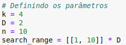
Note that we’re using the same operating range (search_range) for all variables, which is why I’m multiplying by the dimension. But again, this isn’t a rule; each variable could have a different range.

Below is the result of the start_population module:

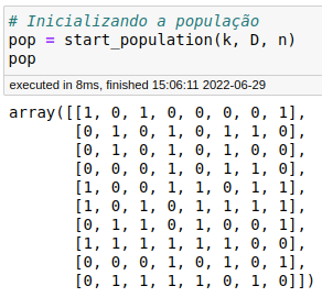
Perfect, given the parameters, our matrix should have 10 rows corresponding to \(n\) and 8 columns corresponding to \(k * D\).

Below is the result of the binary_to_decimal module:

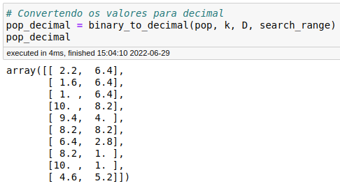
Perfect again! Everything is right with our implementation.

Final Considerations

All the codes implemented here can be found in the repository I created for this series of articles, link here.

At the end of the series, we’ll organize the implemented modules into a class, so don’t worry about that for now.

Did you notice that I didn’t put comments in the code, just a docstring? That’s your task: add comments to the code showing that you understand what each line is doing.

What Will We See in Part 4?

• Evaluation function
• Parent selection
• Crossover and mutation operators

See you next time!