What Needs to Be Done
The objective of the practical work is to implement and evaluate information retrieval models using the FAISS (Facebook AI Similarity Search) similarity search library. The implementation should be done according to the following instructions:
- For result evaluation, use the CFC (Cystic Fibrosis) reference collection. For the result template of this collection’s queries, ignore the relevance score, and consider all documents in the result as relevant. For indexing the CFC collection documents, create a single field by concatenating the texts contained in the AU, TI, SO, MJ, MN, and AB/EX attributes. Perform text preprocessing if necessary.
- To vectorize the documents (and queries), use two different embeddings encodings: TF-IDF and Sentence Transformers.
- For indexing the documents, try one or more indices available in FAISS.
- To perform the queries and obtain their results, use cosine similarity.
- For result evaluation, create a module to return the following metrics. The module should take as input the identification of the queries along with the identifications of the documents in their results, as indicated by the reference collection template and your algorithm, ordered by relevance, and return values for the Precision and Recall metrics. The module should generate the Precision x Recall table for 11 levels of recall so that a single chart can be created with the average values across all queries in the collection. In addition, also calculate the values for the P@5 and P@10 metrics, the average MRR(Q) considering threshold Sh = 5, and plot the Precision-R histogram for the first 20 queries.
- Evaluate each embedding encoding separately, present their respective Precision x Recall charts, and show the results for the other metrics described above.
1. Introduction
Information Retrieval (IR) is a field of computing that explores techniques for representing, storing, organizing, and accessing information. The main objectives of this field are to propose and develop good techniques for text indexing and query mechanisms to search for information in a document collection (Baeza-Yates et al. 1999).
IR models aim to satisfy user needs by retrieving documents that meet their requests. To do this, these models assign a numerical score to each document and rank them according to this score. This score indicates the document’s degree of relevance to the user’s query (Singhal et al. 2001).
This work presents a comparison of some modeling techniques applied to the Cystic Fibrosis collection. This collection contains 1,239 documents published between 1974 and 1979, as well as other data related to each of these publications.
Section 2 discusses the text vectorization representation techniques used. Section 3 presents the combinations of techniques used to compose each strategy. Section 4 describes the hardware and tools used. Section 5 presents the results obtained. Finally, Section 6 concludes the results obtained.
2. Vector Representation
Search engines can be defined, according to (Croft et al. 2010), as the use of information retrieval (IR) techniques for text collections. For the development of a search engine system, it is necessary to define the type of vector representation to be applied to the documents in the collection. There are various ways to generate these representations, ranging from term frequency strategies to machine learning-based strategies.
Term Frequency – Inverse Document Frequency (TF-IDF) is a technique within vector modeling that produces a vector representation of a text, and this strategy is based on weights. The TF component is based on the frequency of each word in each document in the collection, while the IDF component relates to the number of documents in which a word appears (Croft et al. 2010).
A document can be represented by the vector $\vec{d_j} = (w_{1,j}, w_{2,j},…, w_{i,j})$, where the $tf$ component of term $k_i$ in document $d_j$ can be obtained by:
Where $f_{i,j}$ represents the occurrence frequency of a term $k_i$ in document $d_j$. The IDF can be obtained by:
Where $N$ is the total number of documents in a collection, and $n_i$ is the number of documents where term $k_i$ appears. Therefore, the combination of the TF and IDF components produces weights as shown in the following equation:
Another form of modeling is semantic modeling. One of the more recent techniques of this type of modeling is to use the BERT model (Bidirectional Encoder Representations from Transformers) to produce word vectors that capture their meaning in the context in which they are inserted.
BERT is a pre-trained model developed by Google used for Natural Language Processing (NLP) tasks. The pre-training data used was extracted from the BooksCorpus (800 million words) and Wikipedia (2.5 billion words) (Devlin et al. 2018).
However, BERT is limited to word vectorization, so to scale the same concept and generate vectors (embeddings) for an entire sentence, (Reimers and Gurevych 2019) proposed a modification of this model, giving rise to sentence-BERT. The authors explain that sentence-BERT uses an encoder that can convert longer text passages into vectors. This system is very useful for semantic document search since semantically similar sentences are close to each other in the vector space.
3. Adopted Strategies
To proceed with the comparison of the search models, eight combinations of approaches were used, that is, eight search model strategies were implemented. Figure 1 presents a complete flowchart with all the approaches used to compose the adopted strategies.
All strategies go through the stages listed in Figure 1, differing in the approaches used. The strategies are:
- No preprocessing, vectorization via BERT, and Flat indexing;
- No preprocessing, vectorization via BERT, and IVFFlat indexing;
- Word normalization, vectorization via TF-IDF, and Flat indexing;
- Word normalization, vectorization via TF-IDF, and IVFFlat indexing;
- Stopword removal, vectorization via BERT, and Flat indexing;
- Stopword removal, vectorization via BERT, and IVFFlat indexing;
- Word normalization, stopword removal, vectorization via TF-IDF, and Flat indexing;
- Word normalization, stopword removal, vectorization via TF-IDF, and IVFFlat indexing;
In the preprocessing stage, two approaches were used: normalization and stopword removal. The first approach was applied by converting all characters to lowercase. For the second, any word present in the text and in the stopword set was removed from the documents. The stopword set used is available in the NLTK library.

Figure 1. Adopted Approaches in the Applied Strategies
Two approaches were adopted for document vectorization: TF-IDF and sentence-BERT. TF-IDF was applied using the Scikit-Learn library. To generate the embeddings via BERT, the pre-trained model multi-qa-mpnet-base-dot-v11 was used. This model was fine-tuned for semantic search using 215 million question-answer pairs from various sources and supports sentences of up to 512 words, generating an embedding of 768 dimensions.
Two types of indexing were applied: Flat and IVFFlat, both available in the FAISS library.
Flat indexing search is conducted by calculating the similarity between all documents and the query. IVFFlat indexing, on the other hand, clusters documents based on Euclidean distance, with 10 clusters generated in this work. In the IVFFlat search, the query is compared to the centroids of each cluster, and similarity is calculated only with documents present in the cluster to which the query was assigned, thus reducing the search space. The search results using both approaches rank the relevant documents according to the similarity found.
The ranking function to determine the relevance of a document given a query will be obtained using cosine similarity, according to the following equation:
</div> \(\begin{equation} sim(\vec{q}, \vec{d_j}) = \frac{\vec{q} \bullet \vec{d_j} }{|\vec{q}| \times |\vec{d_j}|} \end{equation}\) </div>
The adopted strategies are evaluated through precision, recall, precision in 5 and 10 retrieved documents (P@5 and P@10), precision vs. recall curve, precision-R histogram, and Mean Reciprocal Rank.
4. Experiments
All the libraries mentioned in Section 3 are available for Python, and therefore, all experiments were conducted using this language. The FAISS library, which provides indexing and search options, is available for execution via CPU or GPU processing; in this work, CPU processing was used. Consequently, the configuration of the machine used is: Ryzen 5 3600 processor, 6-CORE, 12-THREADS, speed of 3.6GHz, and two DDR4 RAMs of 16GB each with a speed of 2666MHz.
All the codes used to perform the experiments mentioned in this work can be accessed on GitHub.
5. Results
The vectors produced by sentenceBERT have 768 dimensions, while those produced by TF-IDF have 13,171 dimensions for documents without preprocessing and 13,141 dimensions for documents with stopword removal.
Among the 1,239 documents, 79 were truncated for the documents that did not undergo preprocessing (6.4%) and 25 for the documents from which stopwords were removed (2%).
Figure 2 presents the boxplot of the precision results for the adopted strategies. This chart allows for a visual summary of the precision statistics for all queries. The average precision ranged from 20.1% for IVFFlat indexing, vectorization with TF-IDF and stopword removal, to 27.1% for Flat indexing, vectorization with BERT without preprocessing.
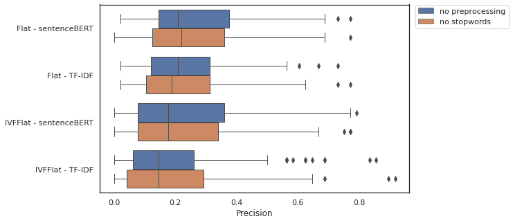
Figure 2. Precision
Comparatively, a two-tailed t-test for the means of two independent samples was used to identify if there is a statistical difference in the experiments conducted with and without the removal of stopwords. The null hypothesis for this test is that the two independent samples have identical mean values. In all cases, the observed p-value was greater than 5% (95% confidence interval), which means we cannot reject our null hypothesis.
Figure 3 presents the recall results. The t-test was implemented with the results obtained, and similar to what was observed with precision, no statistical difference (p-value > 5%) was detected between the strategies using or not using the removal of stopwords.
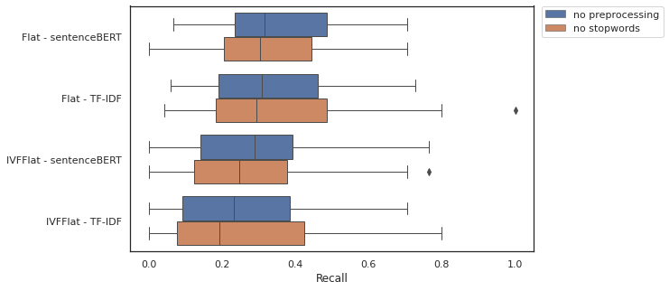
Figure 3. Recall
The precision vs. recall curves are presented in Figure 4. This chart is generated from the average precision obtained for the 11 levels of recall (from 0% to 100%). The chart on the left shows the results for the strategies with vector generation from documents without preprocessing, while the chart on the right shows the results for the strategies that used texts with stopwords removed. It can be observed that the precision values of the strategies at the higher levels of recall (>60%) reverse in the two charts. While the strategy represented by the black line finishes with 100% recall and precision greater than 10% on the left chart, on the right chart, the same strategy finishes with precision less than 10%. This same pattern can be observed in the other strategies.
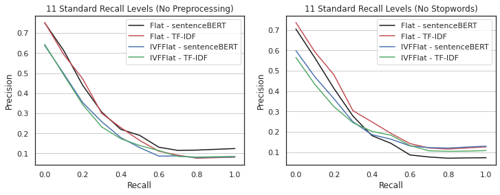
Figure 4. Precision vs Recall
Figures 5 and 6 present the violin plot for the precision results in 5 and 10 documents, respectively. This chart displays a statistical summary and the distribution of the results. In most cases, it is possible to see that there is no difference in the quartiles for the distributions in blue (no preprocessing) and gray (no stopwords), which is corroborated by the results of the t-test, where in all cases the p-value > 5%.
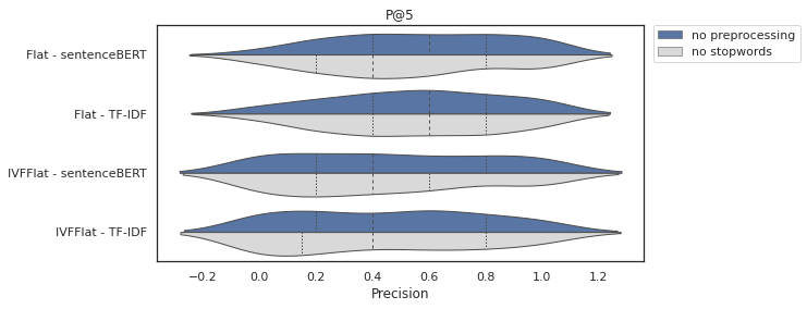
Figure 5. Precision in 5 Documents
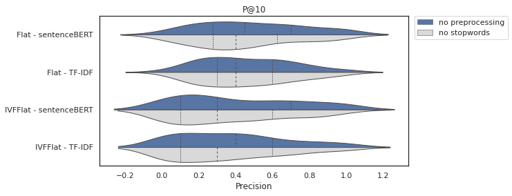
Figure 6. Precision in 10 Documents
The MRR (Mean Reciprocal Rank) is presented in Figure 7. It is noticeable that with the use of documents from which stopwords were removed, fewer relevant documents were retrieved in the top positions, and more queries resulted in no relevant documents within the first five positions. This was observed in all strategies, except for the strategy that uses Flat indexing and TF-IDF vectorization.
![]()
Figure 7. Mean Reciprocal Rank (MRR)
Considering the average results presented so far, two strategies have shown to be more robust given the conditions of the experiment. The first is Flat indexing with BERT vectorization without preprocessing, and the second is the combination of Flat indexing with TF-IDF vectorization and the removal of stopwords. Figure 8 presents the precision-R histogram for the first 20 queries. It is observed that the first strategy has higher precision than the second in 50% of the queries, the second in 30% of the queries, and there is a tie in 20% of the queries.
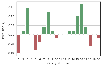
Figure 8. Total Execution Time of the Queries
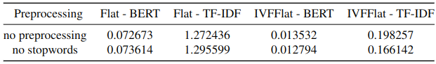
The last factor evaluated was the execution time of the 1,239 queries for each of the strategies. Table 1 presents the times in seconds. It is noted that the strategies using IVFFlat indexing were on average 6.5 times faster compared to Flat indexing. Regarding the type of vectorization, the speed gain provided by IVFFlat indexing compared to Flat was greater in TF-IDF vectorization, with a gain of 7.1x, while in BERT vectorization, the gain was 5.8x.
Tabela 1. Total Execution Time of the Queries
6. Conclusion
Among all the strategies used, the one that achieved the best overall results was the strategy that combined Flat indexing with vector representation via sentenceBERT. However, the search time in this type is directly proportional to the size of the collection. That is, using this type of search is advantageous when precision is more important than speed and/or when the size of the collection is small.
As observed, statistically, there was no difference in the results for the experiments conducted here, whether applying stopword removal or not applying any preprocessing technique.
The FAISS library proved to be a good tool for indexing and searching documents. Its greatest quality is the ease of implementation, requiring only a few lines of code to develop this stage.
References
Baeza-Yates, R., Ribeiro-Neto, B., et al. (1999). Modern information retrieval, volume 463. ACM press New York.
Croft, W. B., Metzler, D., and Strohman, T. (2010). Search engines: Information retrieval in practice, volume 520. Addison-Wesley Reading.
Devlin, J., Chang, M.-W., Lee, K., and Toutanova, K. (2018). Bert: Pre-training of deep bidirectional transformers for language understanding. arXiv preprint arXiv:1810.04805.
Reimers, N. and Gurevych, I. (2019). Sentence-bert: Sentence embeddings using siamese bert-networks. arXiv preprint arXiv:1908.10084.
Singhal, A. et al. (2001). Modern information retrieval: A brief overview. IEEE Data Eng. Bull., 24(4):35–43.